Segmented Interval Method
Overview
The segmented interval method is the core computational approach used in this MSHX implementation. It rigorously handles multi-stream heat exchange, non-constant properties, and phase change by dividing each stream's enthalpy range into discrete intervals and performing thermodynamic flashes at each point (Kamath et al., 2012).
Motivation
Classical LMTD and e-NTU methods assume:
- Constant \(U\) and \(c_p\) along the exchanger
- Single-phase operation (no phase change)
- Only 2 streams
Real industrial MSHXs violate all three assumptions. The segmented interval method removes these limitations.
Algorithm
Step 1: Build H-T Curves
For each stream \(i\), the enthalpy range from inlet to outlet is divided into \(N_{\text{seg}}\) equal intervals. At each enthalpy point, a pressure-enthalpy (PH) flash determines the temperature:
where:
The cumulative heat duty at each point is:
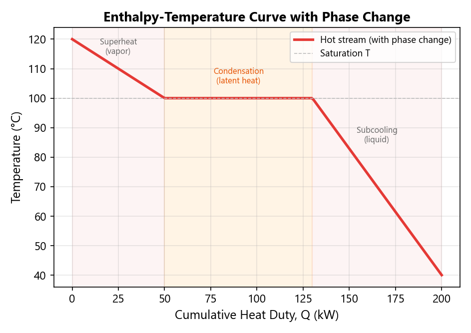
Phase Change Handling
When a stream undergoes phase change, the PH flash returns the saturation temperature for the two-phase region. This creates a flat segment in the H-T curve where temperature remains constant while enthalpy changes — correctly capturing latent heat effects.
Step 2: Build Composite Curves
Individual stream H-T curves are combined into hot and cold composite curves. For multiple streams on the same side:
- Collect all unique temperature breakpoints from all stream curves
- At each temperature \(T\), interpolate the cumulative \(Q\) from each stream's H-T curve
- Sum the contributions: \(Q_{\text{composite}}(T) = \sum_i Q_i(T)\)
This process is detailed in Composite Curves.
Step 3: Zone-by-Zone UA Calculation
The heat transfer area is divided into \(N_{\text{zones}}\) zones of equal fractional heat duty. In each zone:
- Sample the hot composite temperature at fraction \(f\)
- Sample the cold composite temperature at the corresponding fraction (accounting for flow direction)
- Compute the temperature difference \(\Delta T\)
- Calculate the local LMTD and zone UA contribution
For counterflow, both composites are sampled at the same fraction \(f\):
[ T_{\text{hot}}^{(j)} = T_{\text{hot,composite}}(f_j \cdot Q_{\text{hot,total}}) ] [ T_{\text{cold}}^{(j)} = T_{\text{cold,composite}}(f_j \cdot Q_{\text{cold,total}}) ]
For co-current, the cold composite is sampled in reverse:
Step 4: MITA Determination
The minimum internal temperature approach is found by scanning all zone boundaries:
Convergence
The segmented interval method is embedded within a Q-bisection loop that iterates on the total heat duty:
graph TD
    A[Set Q_lo = 0, Q_hi = Q_max] --> B[Q_trial = midpoint]
    B --> C[Distribute Q among streams]
    C --> D[PH flash → outlet T for each stream]
    D --> E[Build H-T curves]
    E --> F[Build composite curves]
    F --> G[Calculate UA and MITA]
    G --> H{Converged?}
    H -->|No| I[Bisect: adjust Q_lo or Q_hi]
    I --> B
    H -->|Yes| J[Done]
Convergence criteria:
| Mode | Criterion | Tolerance |
|---|---|---|
| UA | \(\|UA_{\text{calc}} - UA_{\text{spec}}\| / UA_{\text{spec}} < 0.001\) | 0.1% |
| MITA | \(\|\text{MITA}_{\text{calc}} - \text{MITA}_{\text{spec}}\| < 0.01\) K | 0.01 K |
| Q bounds | \(\|Q_{\text{hi}} - Q_{\text{lo}}\| / Q_{\text{hi}} < 10^{-5}\) | 0.001% |
Maximum iterations: 300.
Number of Segments
The NumberOfSegments parameter (default: 25) controls the resolution of the H-T curves. More segments provide:
- Better resolution near phase boundaries
- More accurate MITA determination near pinch points
- Smoother composite curves
Recommended Values
- 10–20: Quick estimates, single-phase systems
- 25–50: General use (default)
- 50–100: Systems with phase change or tight pinch points